Doubled barbell - further visualizations
[1]:
# Not really required
import sys
sys.path.insert(0, '../../..')

from pyLDLE2 import visualize_all
visualize_all.visualize('../data/pyLDLE2/doubled_barbell/ldle.dat')
matplotlib.get_backend() = module://matplotlib_inline.backend_inline
##################################################
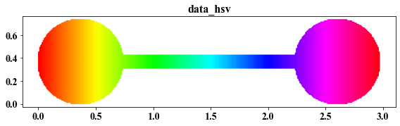
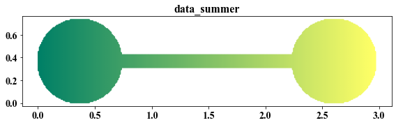
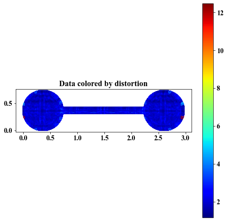
Data
##################################################
Eigenvalues
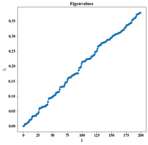
##################################################
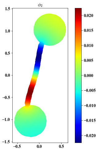
Eigenvectors on data
##################################################
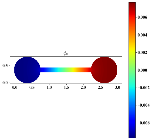
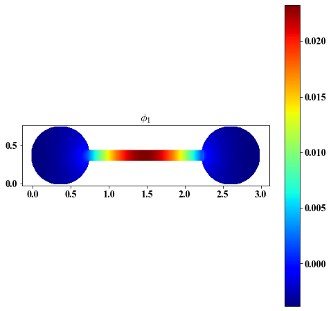
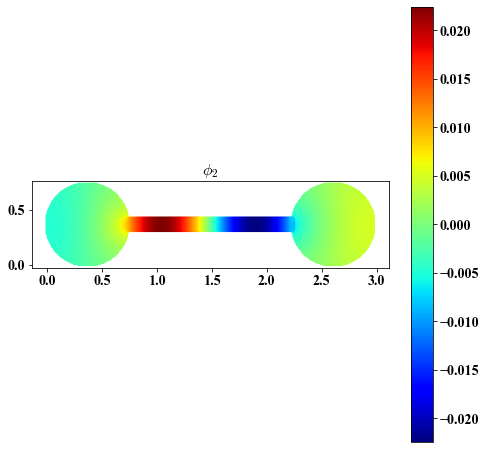
##################################################
Eigenvectors on embedding
##################################################
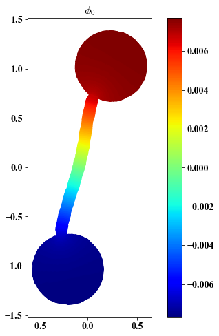
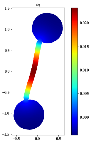
##################################################
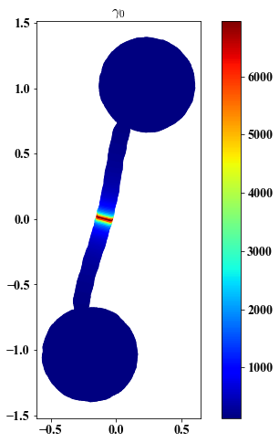
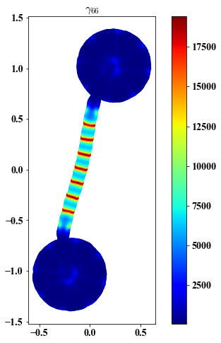
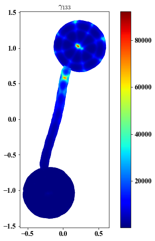
gamma on data
##################################################
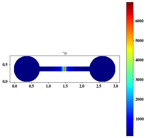
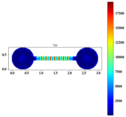
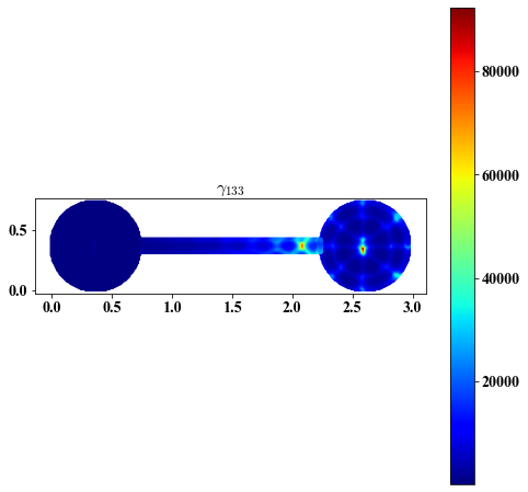
##################################################
gamma on embedding
##################################################
##################################################
No. of eigenvectors with small gradients at each point - possibly identifies boundary
##################################################
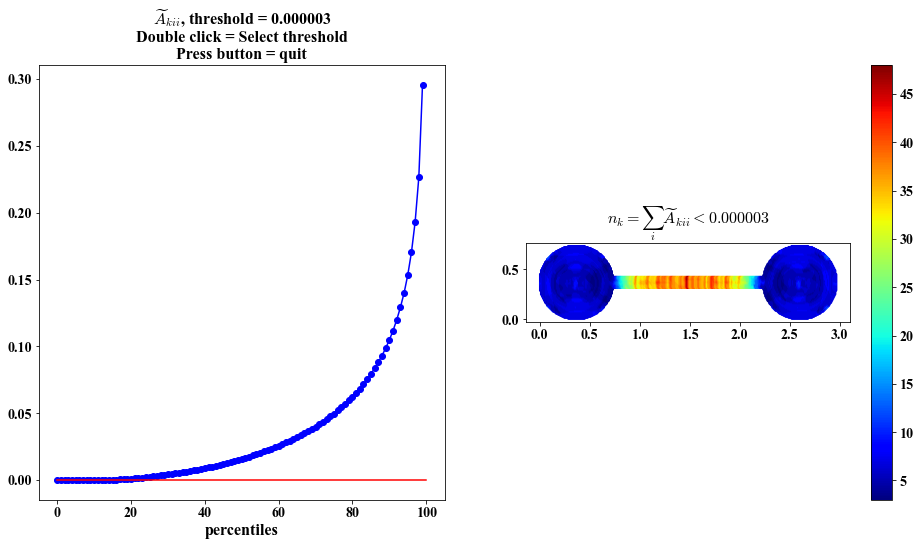
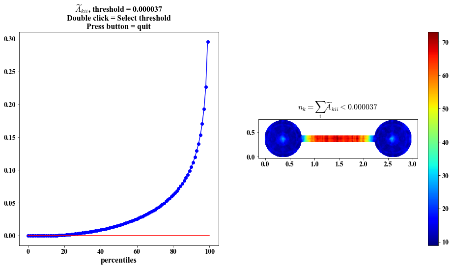

##################################################
Same visualization as above but plots based on the embedding
##################################################
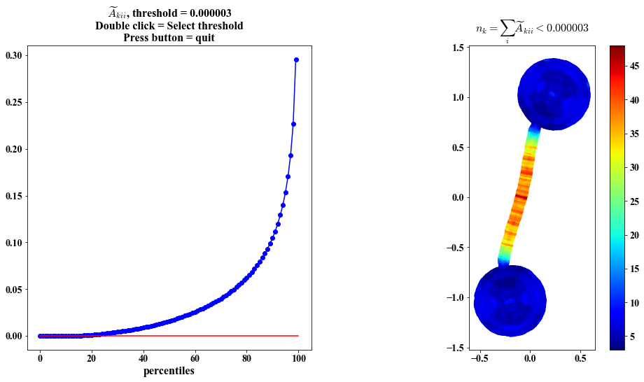
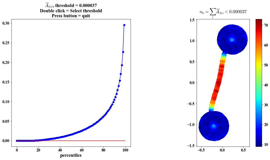
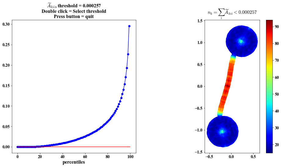
##################################################
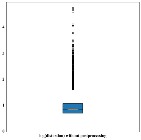
Distortion of local parameterizations without post-processing
##################################################

##################################################
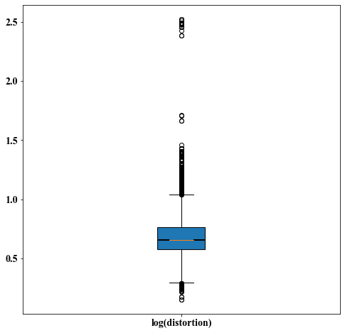
Distortion of local parameterizations with post-processing
##################################################

##################################################
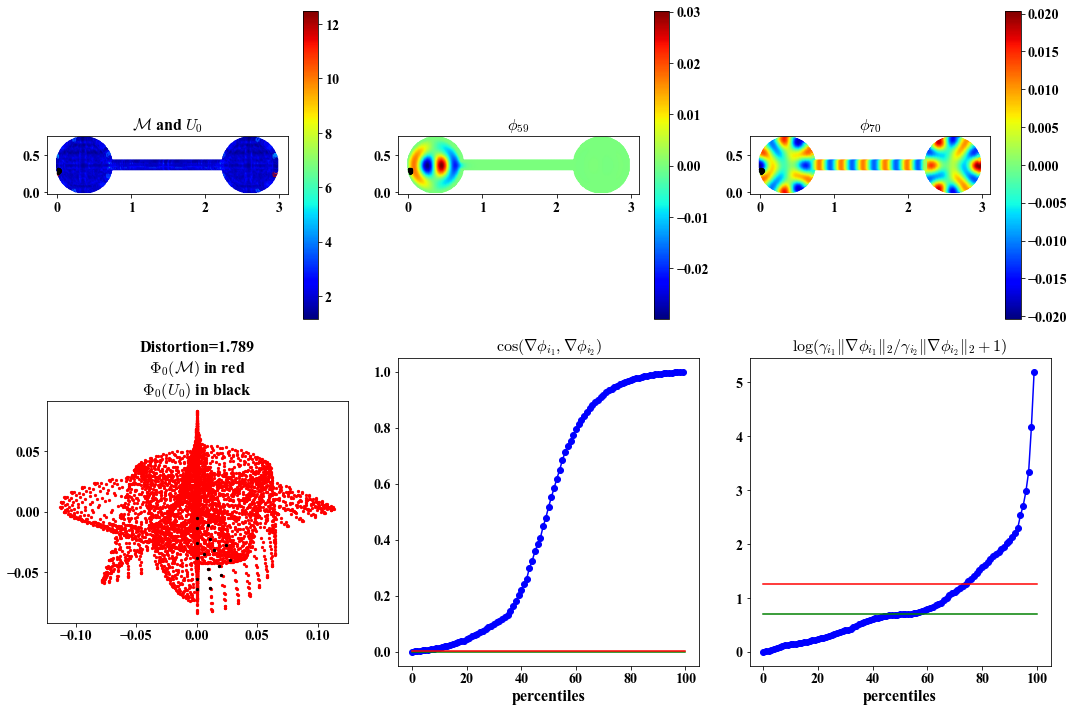
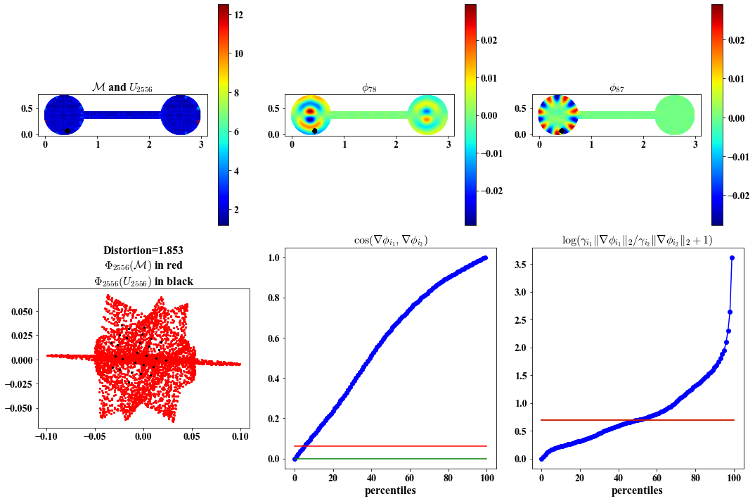
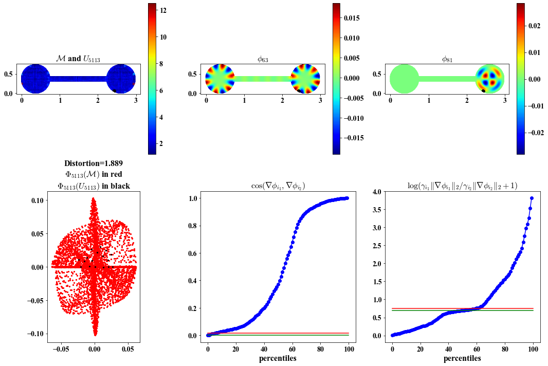
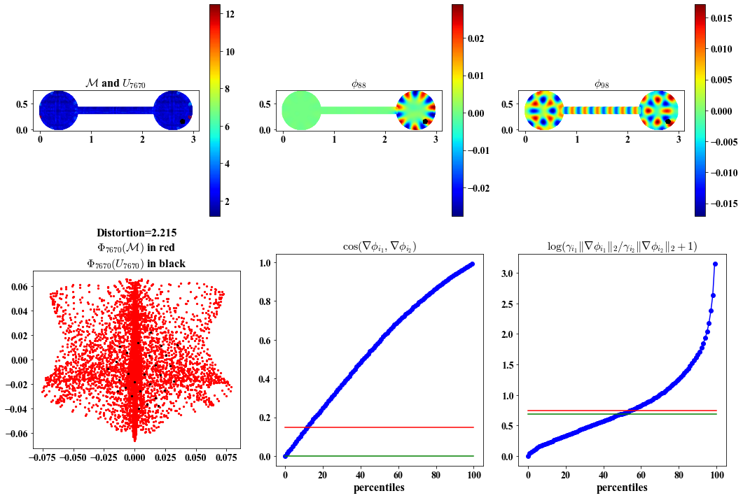
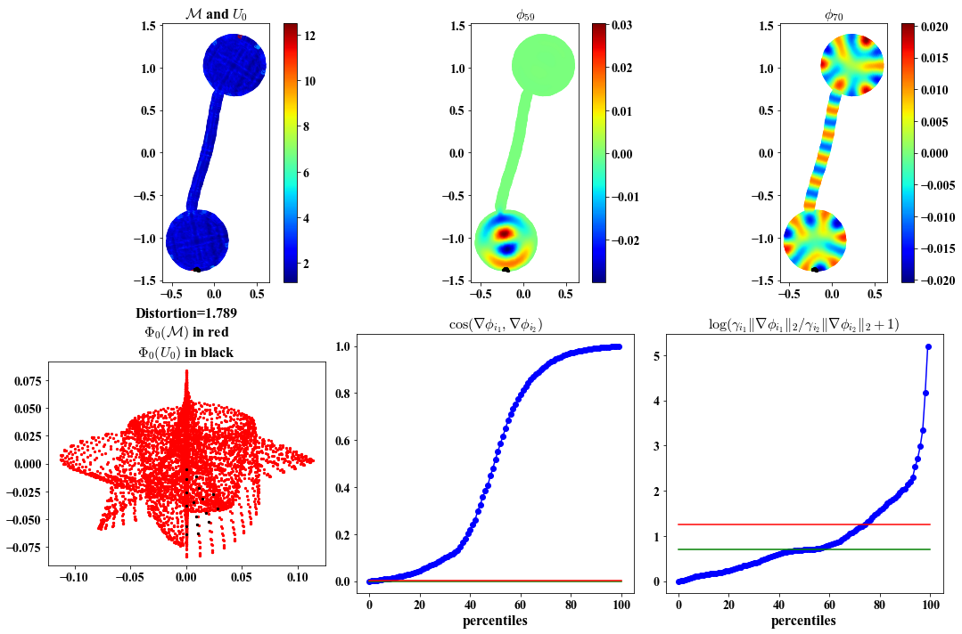
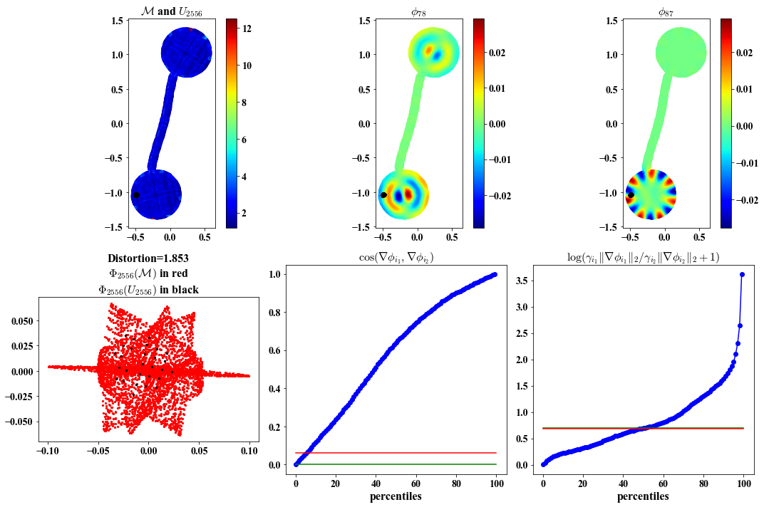
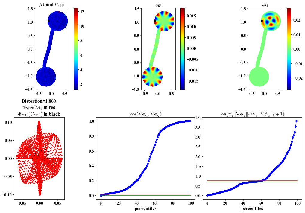
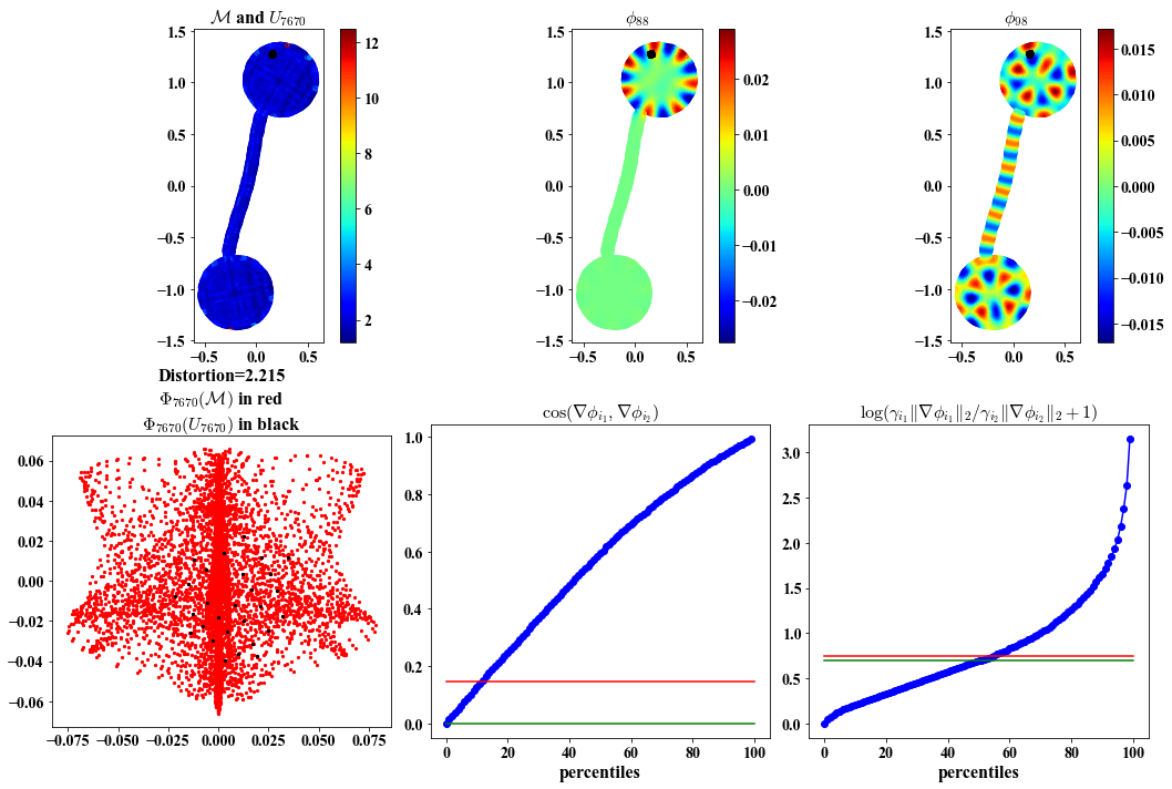
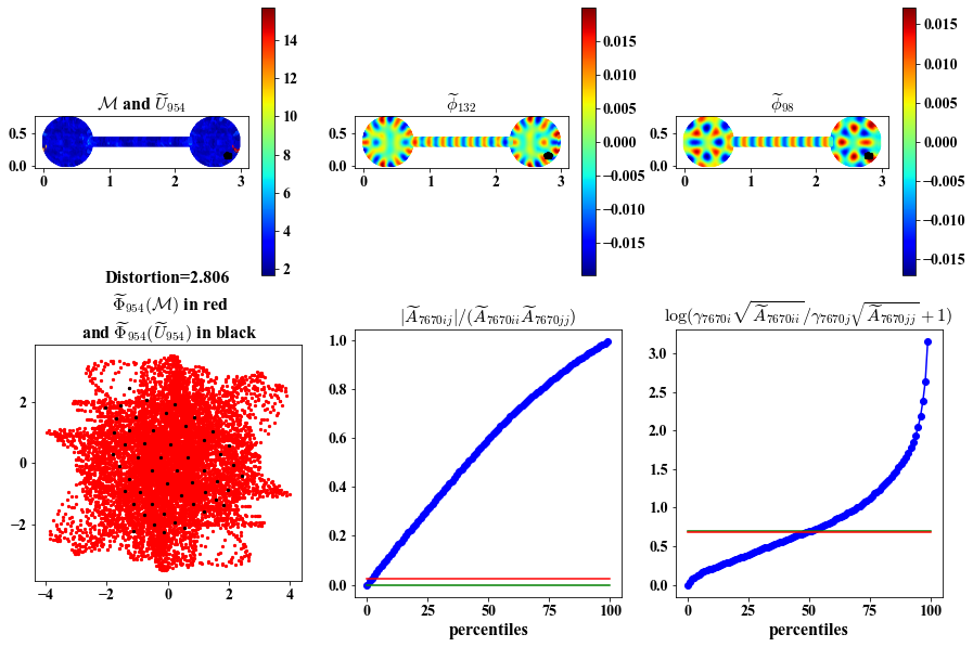
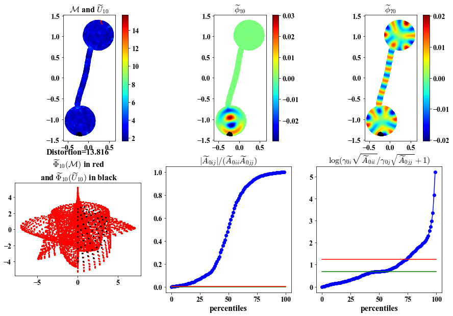
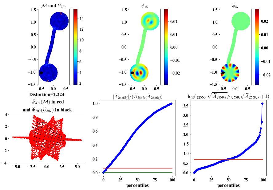
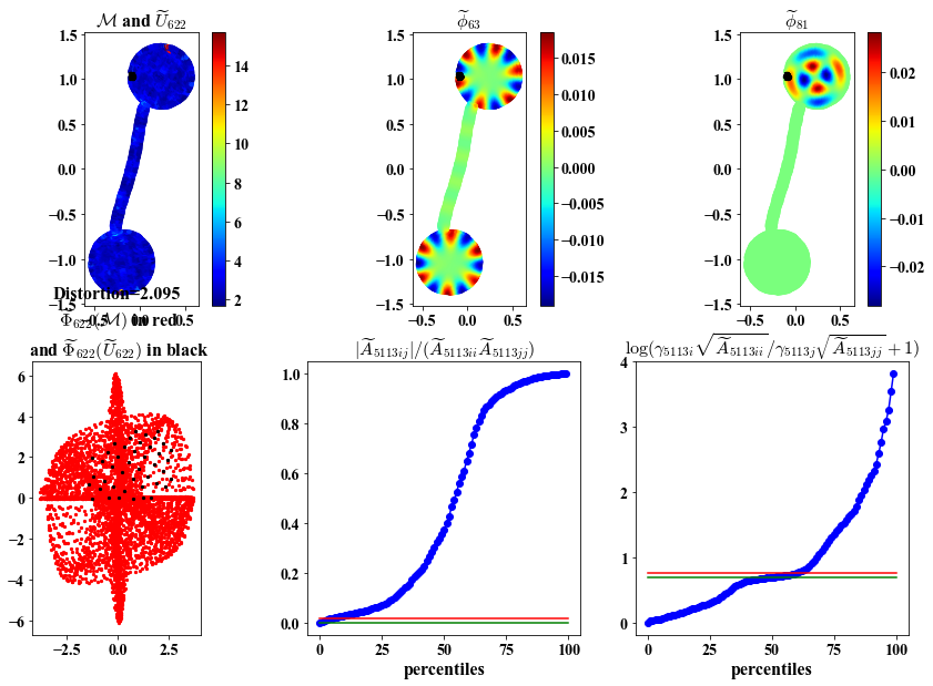
Here we visualize:
1. Local views in the ambient and embedding space.
2. Chosen eigenvectors to construct the local parameterization.
3. Deviation of the chosen eigenvectors from being orthogonal and having same length.
##################################################
##################################################
Same visualization as above but plots based on the embedding.
##################################################
##################################################
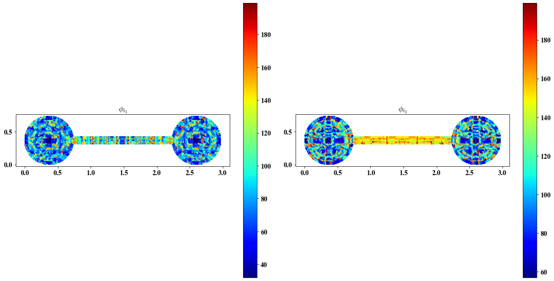
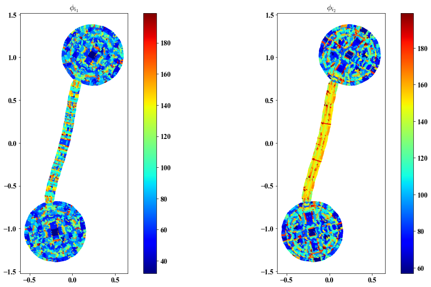
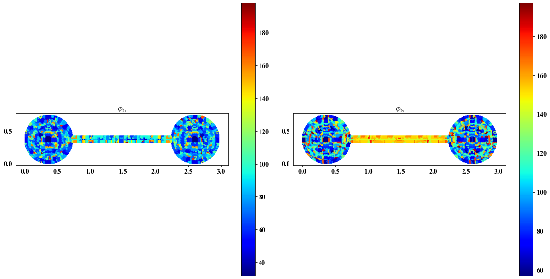
Chosen eigenvectors indices for local views
##################################################
##################################################
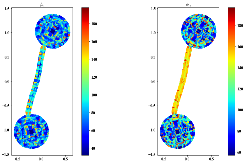
Same visualization but plots based on embedding
##################################################
Sequence of intermediate views
##################################################
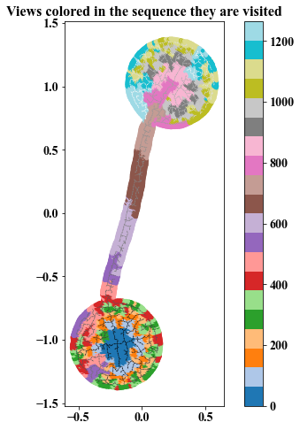
##################################################
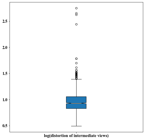
Distortion of intermediate views
##################################################
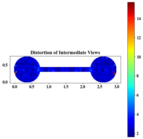
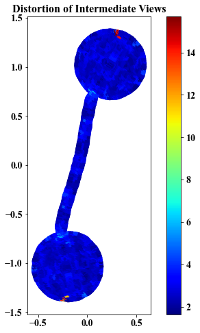
##################################################
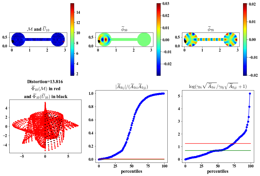
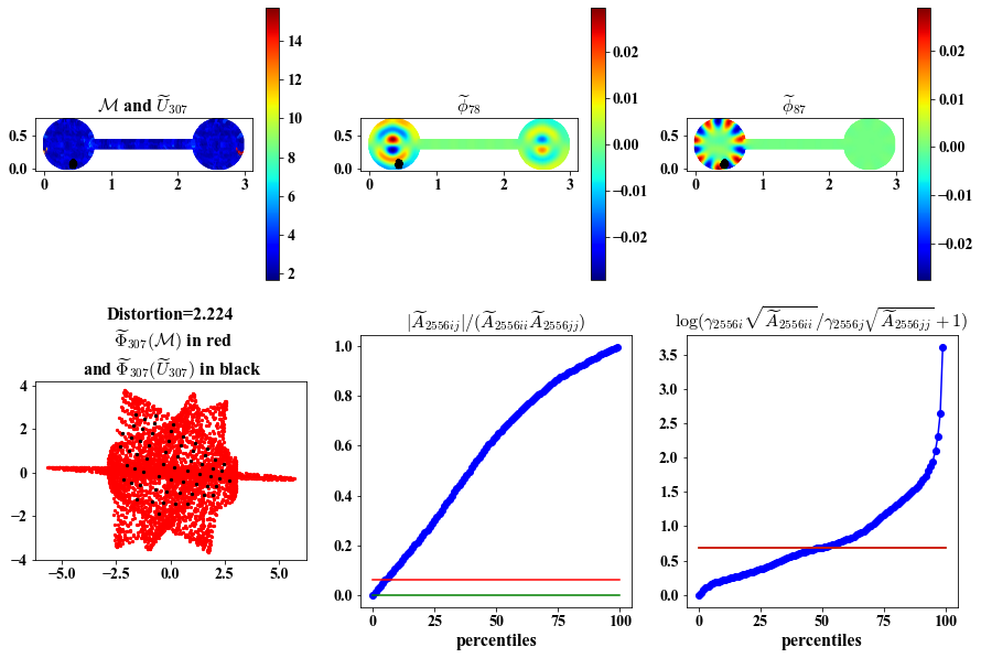
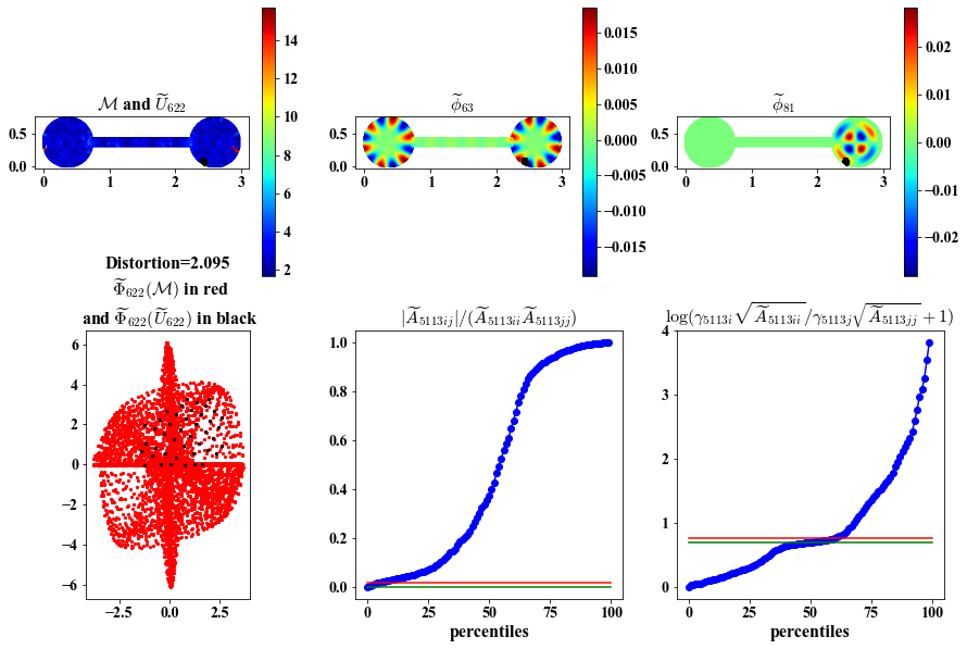
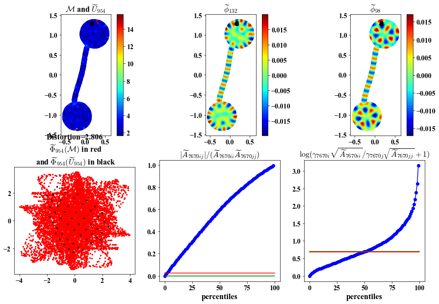
Here we visualize: 1. Intermediate views in the ambient and embedding space.
2. Chosen eigenvectors to construct the intermediate parameterization.
3. Deviation of the chosen eigenvectors from being orthogonal and having same length.
##################################################
##################################################
Same visualization as above but plots based on the embedding
##################################################
##################################################
Chosen eigenvectors indices for intermediate views
##################################################
##################################################
Same visualization but plots based on embedding
##################################################
initial global embedding
##################################################
##################################################
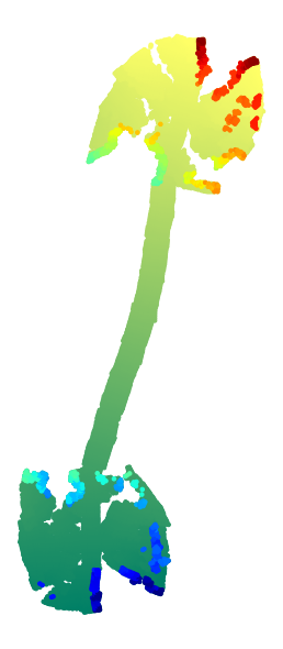
final global embedding
##################################################

[ ]: